Dynamic Programming

AlgorithmsCodingPDEsStochasticProcessesOptimization Fundamentally, dynamic programming is an algorithmic design paradigm that builds upon recursion by storing the results of previously solved subproblems, called memoization. A problem can be solved by dynamic programming if it’s subproblems exhibit the following properties:

1. Repeated subproblems: the problem is solved by reusing solutions of subproblems multiple times
2. Optimal substructure: an optimal solution can be constructed from optimal solutions of subproblems

Equivalently, these criteria can be defined in terms of a computation DAG (no infinite loops) :

1. Repeated subproblems: is not a tree
2. Optimal substructure: the optimal solution can be computed by combining solutions at each solved in reverse topological order

An example is computing the 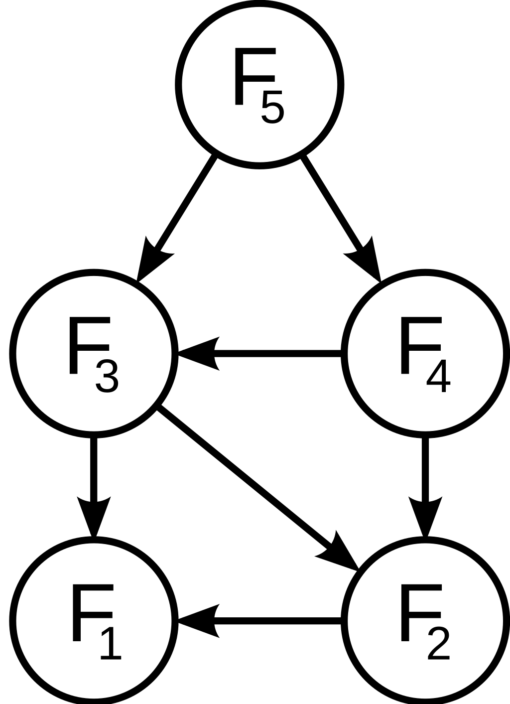-element of the Fibonacci sequence: with computation graph where each (non-leaf) node has two outgoing edges but is not a binary tree, indicating overlapping subproblems ( requires and , which also requires ):

The two approaches to reusing solutions of subproblems are

• Top-down (Recursive DFS + memoization): One first checks whether the solution to a subproblem has been computed and then either utilizes or computes it (as needed) and memoizes it in a table

global mem = [-1]*(n+1)
mem[0], mem[1], 0, 1

def fib(n):
	if mem[n] == -1:
		mem[n] = fib(n-1) + fib(n-2)
	return mem[n]

• Bottom-up (Iterative DFS + memoization): First solve the subproblems and use those solutions to build to solution to bigger subproblems

global mem = [-1]*(n+1)
mem[0], mem[1], 0, 1

def fib(n):
	for i in range(2,n+1):
		mem[i] = mem[i-1] + mem[i-2]
	return mem[n]

If you can work your way backwards to or forwards from then you can use either a top or bottom down approach, however the bottom-up approach allows one to determine the order of computations exactly.